
How To Use Excel Countif Function In Excel
Excel Countif function is a very powerful function in excel especially if you are working with numerous number of data in a database. People can use countif function according to their necessity but today I am going to show how Excel countif function can be used to check and match data in one column to another. This excel countif function is so interesting that it can be used as a powerful database function. In this very article I am going to cover another powerful and simple excel function which you might or might not be aware off.How countif function works
Let’s start
the tutorial about countif function basically important for database clerks,
accountants, bookkeepers as well as to an auditor.

From the
figure above,
Column A
contains some random names. Similarly Column
C also contains some random name but you can see that in this column there are
some names common to the Column A. Now you may ask what are we going to do with
this??? Let’s get in, Over here we are
using excel countif function to check which of the cell in “Column C”
contains the name from “Column A”.
Create a
random column, over here in this tutorial I am choosing “Column E” to insert my
excel countif function.
From the
figure, I inserted excel countif function in “Column E3” as: =countif($A$3:$A$11,C3)
What I did
was, I fixed the Range with $ sign, $ sign is used to fix the cell i.e. if you
want to fix A3 in carrying out any of the calculations, you can do it by using
the $ sign as $A$3. Now I have covered a range which is ”A3 to A11” and it is fixed. Then, I typed C3 as my criteria i.e. it will search if there is a name called “ Raju Dahal” in
the given range of column A. Then
simply, copy the formula in E3 and drag it to E11. What it does is, if the name
in a particular cell in column C has its match in any cell of column A then it
will show “1” in the Column E, if not
then it will show “ 0”.
You can even
select the whole column A(Range) if you don’t want to go with that $ sign as
simply with the formula =countif(A:A,C3). That’s what is did in Column F. The
other process is same as previous.
The next
function, small but interesting function in excel is proper, I don’t want to or
I guess I don’t need to explain what this function does coz, you might already
have figured it out by looking at the figure.
Match the
format of the names in “Column C” with “Column G”. What I did was, just
inserted a proper function with =proper(C3) in “Column (G3)” and drag that to
G11. You can see the difference.
If you have
any questions regarding these two functions then you can always comment on the
comment box, I shall be answering your answers as much as it is possible. If
you like this short tutorial about excel countif function and proper
function, then I shall appreciate if you share this article in any of the
social media and if you don’t want to miss similar tutorials like this you can
always subscribe to by blog through email. Thank you.


0 Comments